Neuromorphic Robot Control: Measuring the Energy–Accuracy Trade-off
Contents
- Define what the controller must preserve
- Separate hardware execution from robot validation
- A comparison of recent experimental conditions
- Treat conversion as a behavioural change
- Optimise the baseline before attributing the gain
- Measure the timing that reaches the actuator
- Pair energy numbers with their measurement boundary
- Calculate energy per successful task
- Understand what the policy can observe
- Include orchestration and state management
- Contact tasks need feedback measurements of their own
- Design trials that expose the trade-off
- A controller-evaluation worksheet
- Advance only when the evidence answers the next question
- References
A robot controller can use less energy per inference and still make the robot use more energy to finish a job. It may need extra corrections, take longer to settle, or require another attempt. Conversely, a small loss of numerical precision may be acceptable if the robot still meets its task tolerance while reducing computation and thermal load.
This is the engineering question behind neuromorphic robot control: does the deployed controller improve a defined application within its actual constraints? Answering it requires measurements across the controller, the interface and the task. Comparing neural-network execution alone is useful, but it cannot determine that outcome.
Recent research supplies several routes into this problem: converting reinforcement-learning policies for Loihi 2, executing spiking controllers on ordinary microcontrollers, and coordinating multiple neural components. This article uses six original studies first released between 8 October 2025 and 8 October 2026. Preprints and their evidence limits are labelled in the references. The evaluation methods proposed below are engineering guidance, not measured OSSI results.
Define what the controller must preserve
Begin with an application requirement, expressed at the robot rather than at the network. For an insertion task it could include successful completion, final alignment, peak contact force and time to completion. For a flying platform it could include attitude tracking, recovery from defined disturbances and operation within the available compute budget.
Identify which deviations are acceptable. A position estimate and an actuator command can tolerate different errors. An intermediate representation might change substantially while the final task remains satisfactory; a small command bias might accumulate into a large final offset. Evaluate the consequences instead of assigning one universal numerical tolerance.
Keep the existing controller as a reproducible reference. Record its configuration, update rate, actuator interface and operating conditions. Decide whether the candidate replaces the whole controller, one estimator, a policy head or a motion cue. An improvement claimed for one component should be reported at that boundary before investigating the complete robot.
Write acceptance criteria before examining candidate results. This reduces the temptation to redefine success around the metric that happens to improve.
Separate hardware execution from robot validation
A study can establish that a network executes on a chip without establishing that it controls a physical robot. Hardware-in-the-loop evaluation is stronger than a pure network simulation, but the environment and plant can still be simulated. Physical component tests establish another useful, narrower result.
Loihi 2 policy-conversion research demonstrates actual neuromorphic execution in a simulated Astrobee control loop. It reports an energy–accuracy trade-off, including larger final errors after conversion; it does not demonstrate neuromorphic flight on the physical Astrobee. 1
This separation should appear in your own test report. Label the execution substrate, plant, sensor inputs and actuator outputs independently. “Real hardware” is ambiguous when the processor is physical but the robot is virtual. “Real robot” is also incomplete when a neural controller runs on a desktop emulator.
Simulated tests are valuable for repeatable disturbance sweeps and regression checks. Physical tests expose effects that the model may omit. Use both, with a clear account of which conclusion each supports and which remaining uncertainty the next stage is intended to resolve.
A comparison of recent experimental conditions
The following research spans controller execution and supporting measurements. It is a conditions map, not a leaderboard: the experiments do not share a robot, workload or system-energy boundary.
| Study | Neural execution and plant | What is evaluated | Material limitation |
|---|---|---|---|
| RL policy on Loihi 2 1 | Actual Loihi 2; simulated Astrobee | Converted policy, inference energy and tracking error | Conversion changes accuracy; simulated plant |
| Flapping-wing SNN 2 | ESP32-S3; physical untethered flight | Onboard estimation/control and embedded inference | Restricted flight tests; power increment excludes complete robot |
| Multi-component control 3 | Loihi replay, simulated insertion, emulated networks on real arm | Orchestration and component behaviour | Full chip-to-robot integration not achieved |
| EventShiftFlow 4 | Single-axis Artix-7 prototype; recorded/synthetic motion | Approximate motion scoring | Tool-estimated power; no closed-loop avoidance task |
| Propeller sensing 5 | Recorded physical quadrotor flights | Frequency and relative-state estimation | No online formation-control demonstration |
| Event-based tactile force 6 | Physical sensor/CNC; desktop CPU/GPU | Force reconstruction | No deployed grasping controller |
A controller project may combine ideas from these studies. The combined system still requires its own validation; complementary component results do not add up automatically to demonstrated autonomy.
Treat conversion as a behavioural change
Converting a trained artificial neural network into a spiking implementation changes the execution path. Quantisation, encoding thresholds, persistent state and decoding may alter the policy's input–output relationship. Evaluate those changes before letting the converted controller command the plant.
Build a replay test that feeds identical observation sequences into the original and candidate implementations. Compare actions in meaningful units. Separate instantaneous differences from sustained bias, and inspect behaviour near command limits, reversals and small corrective motions. Include quiet periods where an event-driven implementation may transmit little information.
Replay agreement alone is insufficient because a closed loop generates its own future observations. A small action difference changes the plant state, which changes subsequent inputs. Follow replay with repeatable simulated closed-loop trials and then controlled physical trials where appropriate.
Sweep conversion parameters against task metrics, not only output similarity. For example, a larger encoding threshold could reduce activity but alter a small correction that matters near the goal. Record the accuracy and resource outcomes of each setting. Keep the chosen configuration, conversion tool version and trained model together so the experiment can be reproduced.
A converted policy is a candidate controller with measurable differences, even when it originated from a successful reference model.
Optimise the baseline before attributing the gain
A comparison should distinguish benefits from the computational approach, software implementation and hardware. An event-driven loop that skips inactive connections may outperform a naïve dense loop without outperforming every optimised alternative.
The flapping-wing study reports physical onboard control and lower inference cost on ESP32-S3. Its headline comparison uses an unoptimised dense FP32 ANN, while supplementary SIMD tests provide a more demanding comparison. The paper also measures extra state memory. 2
For an evaluation, give each candidate reasonable implementation effort. Check vector instructions, quantisation support, compiler options, memory placement and batch size. Match the task and interface even when model architectures differ. If available engineering time limits optimisation, disclose that limit rather than implying a universal architectural advantage.
Keep two comparisons: a controlled one that isolates a specific change, and a practical one against the best feasible deployment baseline. The first explains why performance changes. The second informs purchasing and integration.
Measure accuracy after optimisation as well as speed. Lower precision or different kernels may change controller output. Include memory and scheduling overhead from recurrent or spiking state. A faster inference with a larger memory footprint can be attractive, but its resource trade-off should remain visible.
Measure the timing that reaches the actuator
Controller execution time is only part of a feedback cycle. The input may already be old when inference begins, and the resulting action may wait before reaching the actuator. A controller can run quickly yet operate on stale measurements.
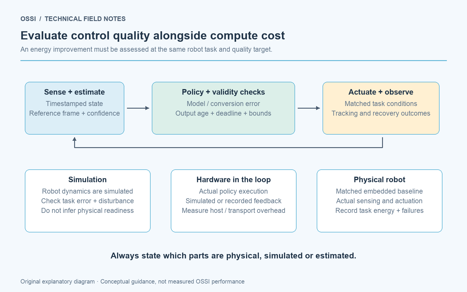
Evaluate the complete feedback cycle, then relate its timing and energy to task outcomes.
Record measurement time, observation delivery, policy start and finish, command publication and actuator consumption. Attach a reference time to the estimated state. If the estimate predicts a future state, document that convention and how its uncertainty is represented.
Report timing distributions rather than only averages. Include the longest observed delay, jitter and missed deadlines under each workload. Identify whether a late command is applied, discarded or replaced by a separately validated fallback. These choices influence closed-loop behaviour.
An illustrative controller executing in 0.8 ms can still receive observations 12 ms old and wait another 2 ms for command delivery. Those assumed values are not OSSI measurements. They show why optimising the 0.8 ms component may produce only a modest change in the delay relevant to the robot.
Pair energy numbers with their measurement boundary
Record where power is measured and what equipment lies inside that boundary. An accelerator estimate, board measurement and robot battery measurement answer different questions. Subtracting idle power estimates an incremental workload cost; it does not describe the total power required to operate the system.
For each result, state the workload duration, sampling method, baseline treatment, included communication and measurement uncertainty. Measure enough repeated runs to see whether the claimed difference is larger than variation. Keep warm-up, idle intervals and reset costs visible.
A tool estimate is useful for design iteration, but should retain that label. EventShiftFlow's single-axis FPGA work illustrates this distinction: its reported power comes from implementation tools, while its prototype establishes a datapath result. Neither establishes total energy for an avoidance manoeuvre. 4
Do not multiply inference energy by an assumed control rate and present the result as complete robot power. Such a calculation can estimate one contribution if its assumptions are explicit. The host, sensors, communications, actuators and any additional processing must be measured or accounted for separately.
For broader reporting conventions, see How to Benchmark Neuromorphic Edge Compute for Robotics.
Calculate energy per successful task
A practical comparison should include complete attempts, including failures and retries. The controller's efficiency matters commercially when it helps the robot complete the required work within the resource budget.
energy per successful task = energy consumed across all evaluated attempts
                             / number of successful completions
Keep this alongside success rate and task duration. It is undefined when there are no successful completions, and it can conceal very different failure patterns unless the underlying results are also reported. Define when each attempt starts and ends, and include recovery according to the intended operating procedure.
Consider an illustrative example, not a measured OSSI result. Controller A consumes 10 J of compute and 90 J elsewhere per attempt, with 90 successful completions from 100 attempts. Controller B consumes 5 J of compute and the same 90 J elsewhere, with 80 successes. Their totals imply approximately 111 J and 119 J per successful task respectively. Lower compute cost has not delivered a lower task cost in this assumed scenario.
Real actuator energy may change with the control trajectory, so holding it constant is only an explanatory simplification. Measure it during physical evaluation whenever task energy is the proposed benefit.
Understand what the policy can observe
A control benchmark assumes an observation interface. Check whether the deployed robot can actually provide those observations with the same units, accuracy and delay. Simulation may expose state directly, while physical deployment requires estimation.
Event-based propeller sensing extracts dynamics from recorded outdoor flights, but its measurements depend on the sensing geometry and available cues. Its estimator result should not be read as complete online control of a multi-robot formation. 5
For your controller, list every observation and its origin. Mark direct measurements, filtered estimates, model predictions and configuration constants. Include observation age and validity. Test missing or intermittent inputs through the same interface used in deployment.
Avoid evaluating the policy with perfect state while quoting the timing and energy of a realistic sensor front end as though both were one tested system. Integrate the estimator and controller, then measure the resulting task behaviour. A policy may need retuning when noise, occlusion or intermittent updates alter the state distribution.
Keep estimator errors and policy errors distinguishable in logs. This lets the team improve the failing component without unnecessarily replacing a successful one.
Include orchestration and state management
A robot rarely executes one isolated neural network. It may alternate between searching, tracking, approaching and interacting, with different components active in each phase. Their coordination consumes resources and introduces failure modes.
Multi-component neuromorphic research demonstrates on-chip orchestration and separate robot experiments, but complete Loihi-to-robot integration was not achieved. It is evidence about a promising architecture and its components, rather than a finished physical control pipeline. 3
Draw your state transitions and identify who owns each transition. Define the conditions that activate an estimator, reset a recurrent state or switch a controller. Record transitions during tests; unexplained resets can make a favourable average timing result difficult to reproduce.
Include startup, failed search, interrupted contact and return-to-home behaviour. A controller that performs well after ideal initialisation may behave differently after a partial attempt. Evaluate state carry-over intentionally rather than letting it depend on whichever process happened to restart.
Measure the host and communications needed to coordinate components. If removing a host is the design goal, verify that sensor handling, failure detection and deployment management still have an implemented owner. On-chip inference does not automatically remove the rest of the software stack.
Contact tasks need feedback measurements of their own
For manipulation, pose accuracy alone may miss the important outcome. A candidate controller can align well but apply excessive contact force, or react late to a changing load. Define contact metrics alongside geometrical ones.
Event-based tactile research reports physical force reconstruction using controlled indentations, with desktop CPU/GPU processing. Validation uses measured net force because dense force ground truth is unavailable; downstream manipulation remains a future step. 6
A controller evaluation should therefore first check the tactile interface: calibration, force units, delay, contact geometry and behaviour during sustained loading. Then test the integrated task with ground truth that addresses the application, such as placement, retention or force excursions.
Treat sensing and control updates separately. A sensor estimate arriving frequently does not guarantee that each estimate changes an actuator command or improves the task. Conversely, a controller may deliberately filter or hold measurements. Log those decisions.
Test slow contact changes, abrupt transitions and loss of contact. The controller needs a clear distinction between a valid low-force measurement and absence of valid data. This is especially important when sparse signals feed a system designed around regular updates.
Design trials that expose the trade-off
Use a staged trial matrix. Begin with nominal cases that verify basic integration, then vary one relevant factor at a time: initial error, observation delay, load, target motion or a defined disturbance. Follow with combined conditions representative of the application.
Use the same cases and initial states across candidates when possible. Record seeds for simulation and explain what repeatability is achievable physically. Separate tuning data from held-out evaluation. A candidate that received extensive task-specific tuning should not be compared with a reference left at unsuitable defaults.
Report per-condition outcomes before aggregating them. Average success can conceal a controller that fails specifically when the payload is heavier or when the sensor stream becomes quiet. Keep failure counts and their denominator visible.
Retain trajectories, commands, validity flags and power traces around failures. Classify whether the immediate cause was inaccurate estimation, policy behaviour, command saturation, delay or a hardware/interface issue. This classification is more actionable than a single score and helps identify whether a hardware change could plausibly fix the problem.
Where measurements disagree with expectation, reproduce the case and examine instrumentation before drawing architectural conclusions.
A controller-evaluation worksheet
Use this worksheet as the minimum brief for a technical comparison. Write an answer and an evidence location for each item.
- Task contract: What constitutes success, and what tolerances define unacceptable behaviour?
- Replacement boundary: Which estimator, policy, controller or coordination component changes?
- Observations: What signals, units, clocks, ages and validity flags are available?
- Actions: What command rate, bounds, actuator interface and late-command policy apply?
- Models: Which weights, quantisation, encoding thresholds and recurrent-state rules are frozen?
- Baselines: Which practical and controlled comparisons have equivalent tuning effort?
- Timing: Which sensor-to-actuator intervals, deadline misses and jitter are measured?
- Resources: What processor, host, memory, communications and power boundaries are included?
- Trials: Which nominal, disturbed and held-out conditions are repeated?
- Outcomes: What success, error, force, duration and energy-per-success metrics are recorded?
- Failures: What recovery, reset and fallback behaviour is evaluated?
- Decision: Which criteria must pass together before the candidate advances?
The worksheet makes an accelerator discussion concrete. A model file alone cannot communicate the feedback problem or the evidence needed to decide whether deployment is worthwhile.
Advance only when the evidence answers the next question
A useful first milestone is faithful execution of the candidate model on the target hardware, with traceable inputs and outputs. The next is acceptable closed-loop behaviour under reproducible conditions. Physical integration then tests sensing, timing, actuation and task outcomes together.
Keep a versioned acceptance report at each stage. Include model and firmware versions, sensor settings, calibration, hardware configuration and test data. A passed report belongs to that configuration and tested envelope; it should not silently extend to a new payload, control rate or encoding threshold.
If a candidate saves inference energy but misses the task tolerance, record that outcome plainly. The next experiment might improve encoding, retrain with deployment effects or change where the candidate sits in the stack. If it passes the task but offers little total-energy benefit, another constraint such as latency or thermal load may still justify it, provided that benefit is measured.
For allocation of neural and conventional processing, see Building a Heterogeneous Robot Compute Stack. The OSSI neuromorphic robotics guide connects control, sensing and measurement across this series.
To evaluate a specific controller or robot, Discuss your robotics workload with OSSI. Share your sensor stream, control deadline, energy budget, compute platform and success criteria. Those details establish the comparison that matters for your application.
References
- Kenneth Stewart, Roxana Leontie, Samantha Chapin, Joe Hays, Sumit Bam Shrestha and Carl Glen Henshaw (2025). Autonomous Reinforcement Learning Robot Control with Intel's Loihi 2 Neuromorphic Hardware. arXiv:2512.03911v1; first released 3 December 2025. Preprint, submitted for NICE 2026 review according to the arXiv record; formal publication not established here.
- Rim El Filali, Chenrui Feng, Chao Gao and Weibin Gu (2026). Spiking Neural Network Control of a Flapping-Wing Robot on Resource-Constrained Hardware. arXiv:2605.19430v3, revised 23 September 2026; first released 19 May 2026 under the title “Neuromorphic Control of a Flapping-Wing Robot on Resource-Constrained Hardware”. Preprint; formal peer-reviewed publication not established here.
- Evan Eames, Priyadarshini Kannan, Ronan Sangouard, Philipp Plank, Elvin Hajizada, Gintautas Palinauskas, Lana Amaya, Michael Neumeier, Sai Thejeshwar Sharma, Marcella Toth, Prottush Sarkar and Axel von Arnim (2026). The More the Merrier: Running Multiple Neuromorphic Components On-Chip for Robotic Control. arXiv:2602.13747v1; first released 14 February 2026. ArXiv records preliminary acceptance at Neuromorphic Computing and Engineering and a related DOI; formal publication date not established here.
- Arianna Alonso Bizzi, Fernando Cladera and C. J. Taylor (2026). EventShiftFlow: Towards Hardware-efficient FPGA-based Flow Estimation. arXiv:2605.28312v1; first released 27 May 2026. Accepted ICRA 2026 workshop paper; formal publication date not established here.
- Ravi Kumar Thakur, Luis Granados Segura, Jan Klivan, Radim Špetlík, Tobiáš Vinklárek, Matouš Vrba and Martin Saska (2026). Relative State Estimation using Event-Based Propeller Sensing. arXiv:2604.18289v1; first released 20 April 2026. Preprint, also listed among accepted ICRA 2026 workshop papers; formal publication date not established here.
- Agis Politis, René Zurbrügg and Valentina Cavinato (2026). Dense Force Estimation with an Event-based Optical Tactile Sensor. arXiv:2606.09451v1; first released 8 June 2026. Preprint; formal peer-reviewed publication not established here.
Discuss your robotics workload with OSSI
Tell us about your platform and where adaptive, event-driven compute could help.
Start the conversation →