How to Benchmark Neuromorphic Edge Compute for Robotics
Contents
- Start with a task contract
- Read the experimental conditions before the headline
- Draw three measurement boundaries
- Build a credible conventional baseline
- Measure observation age and response latency
- Measure energy over the same useful work
- Sweep activity, temporal structure and load
- Treat learning as a separate operating mode
- Connect compute quality to robot behaviour
- Make the experiment reproducible
- A worked decision example
- Benchmark worksheet
- Turn the result into an integration decision
- References
A robotics team evaluating neuromorphic compute needs to answer a practical question: will this processing path improve a particular robot task within its power, timing and quality constraints? A number such as energy per synaptic operation cannot answer that question on its own. Neither can a fast inference kernel if the robot spends most of its response time waiting for data, preparing an input or transferring a result.
The useful benchmark is a contract between the workload and the hardware. It specifies what information arrives, when a decision becomes useful, what counts as a correct result, and which equipment consumes energy to produce it. Once those conditions are explicit, specialist accelerators and conventional embedded processors can be compared without hiding their different strengths.
This article develops a measurement protocol around original research first released between 8 October 2025 and 8 October 2026. The papers demonstrate different stages of maturity: measured neuromorphic hardware, FPGA implementations, tool-based energy estimates and physical onboard control. Their results are valuable because their boundaries can be examined. They are not interchangeable estimates of a robot's battery life.
For an introduction to the underlying concepts, start with the OSSI technical guide to neuromorphic computing for robotics. Here, the emphasis is the engineering work needed to turn a promising result into an evaluation decision.
Start with a task contract
Write the benchmark specification before selecting a processor. Otherwise it is easy to choose a workload that flatters an available implementation.
A task contract should describe the input, output, deadline, quality threshold and operating envelope. For a warehouse motion-estimation module, the input might be timestamped sensor events and inertial measurements; the output might be a motion estimate with uncertainty and an observation interval. The deadline should be tied to the consuming controller. The quality threshold might specify error, coverage and failure rate under defined motion and lighting conditions.
Define the unit of useful work carefully. One event, one neural timestep, one image, one observation window, one decision and one completed manoeuvre are different units. A method can process many events per second while producing an infrequent decision. A controller can generate inexpensive actions while requiring more actions to complete a task. Report the intermediate units when they explain performance, but make the purchase decision using the useful output.
Also fix what the evaluator is allowed to change. A hardware-only comparison holds the model and decision rule as closely matched as possible. A system-design comparison allows each platform a suitable algorithm, provided every candidate meets the same task requirements. Both are useful. They answer different questions, so publish them separately.
Define failure explicitly. An invalid estimate, missing output, deadline miss, rejected action or unfinished manoeuvre must remain in the run record and acceptance statistics. Retain the energy spent on failed attempts when calculating energy per valid decision, and report the fraction of attempted decisions that were valid and timely alongside it.
Read the experimental conditions before the headline
The following comparison identifies the scope of six recent studies. It is a guide to interpreting evidence, rather than a performance ranking.
| Research example | Experimental conditions | Boundary to retain |
|---|---|---|
| CLP-SNN 1 | Loihi 2 continual-learning head; frozen features extracted externally; I/O latency excluded | Learning-head results do not include the complete sensing pipeline |
| CLANE 2 | Loihi 2 action recognition with frozen spiking features and an on-chip learning head | Sequence-processing assumptions and the chosen GPU baseline affect the comparison |
| PYNQ-Z2 deployment 3 | Board-validated MNIST classifier; separate programmable-logic and host-validation timing | Dynamic logic energy is tool-estimated; the validation loop includes reference execution |
| EventShiftFlow 4 | Recorded events; preliminary one-axis FPGA implementation | Scoring latency excludes accumulation; FPGA power is estimated |
| Astrobee controller 5 | Actual Loihi 2 policy execution; robot and environment simulated | Compute evidence is measured; physical robot deployment is not demonstrated here |
| Flapping-wing control 6 | Physical onboard ESP32-S3 control; scalar embedded baselines and SIMD ablation | Reported inference power is an increment above a board baseline |
For papers [1] and [2], the following disclosure applies: This research includes OSSI co-founder Yulia Sandamirskaya as a co-author; its experiments use Intel Loihi 2, not OSSI hardware.
The strongest lesson is methodological. Ask which stages were measured, which stages were estimated, and which parts of the robot existed physically. A paper can provide excellent evidence for an accelerator while leaving substantial integration work open.
Draw three measurement boundaries
Use three nested views: accelerator, processing subsystem and robot task.
The accelerator view starts when a valid input is available at the accelerator interface and ends when its result is available there. Include the execution state required by the deployed method. Identify whether transfers, synchronisation and output decoding are inside this boundary. This view helps a hardware engineer diagnose the implementation.
The processing-subsystem view includes the sensor interface, input conversion, host orchestration, memory movement, inference or learning, and result handling. This is usually the most relevant initial view for selecting a compute module. A processor that remains awake to manage a low-power accelerator belongs in this view.
The task view includes the duration and resources required to achieve the robot objective. Include actuation when making claims about task energy or mission endurance. Record whether a changed controller causes extra travel, corrective movements, slower settling or more retries.
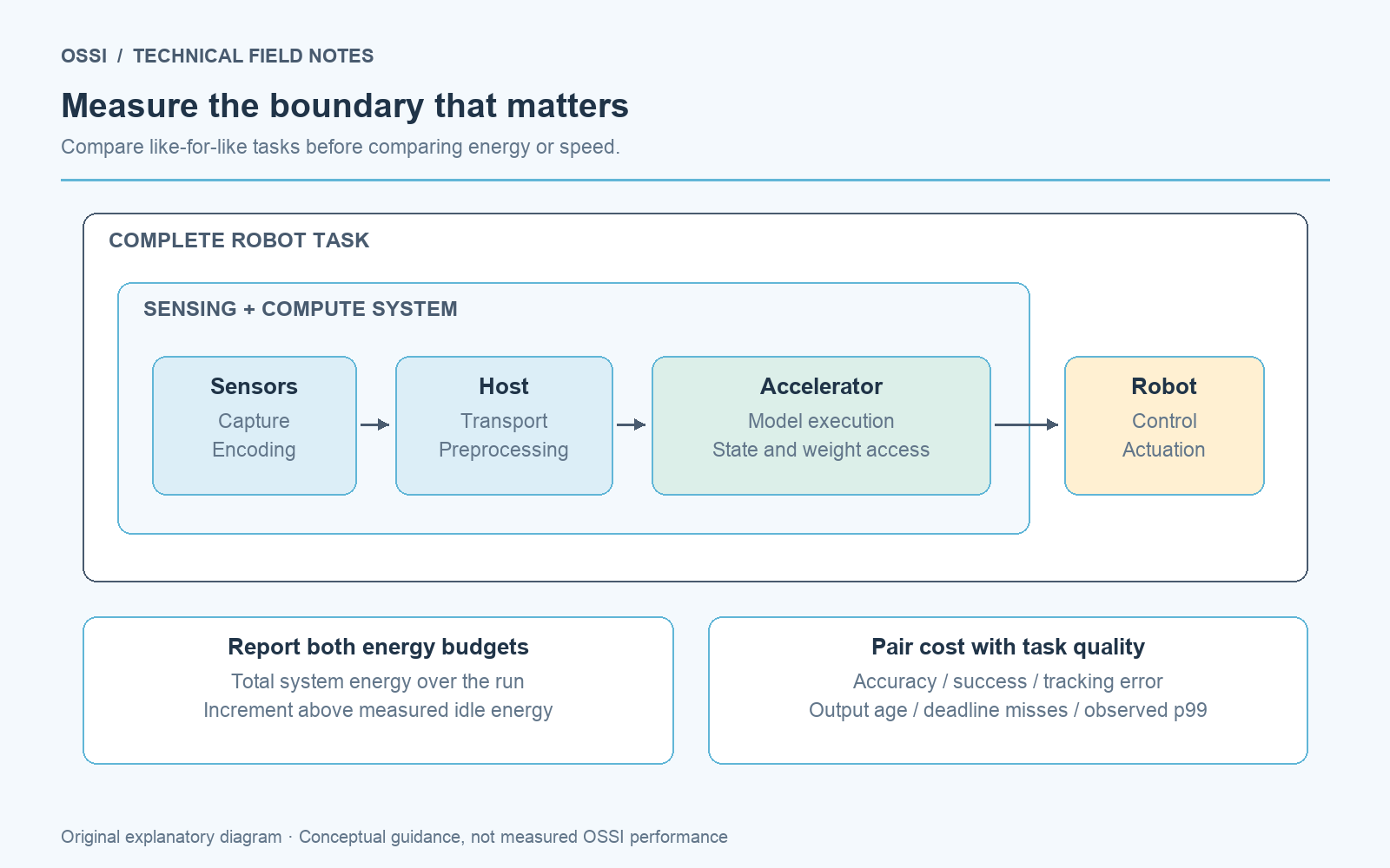
Measure the accelerator, the surrounding processing path and the complete task separately. Attach every reported result to its boundary.
Do not add numbers from nested boundaries: that double-counts shared activity. Instead, measure the larger boundary directly and use stage instrumentation to explain it. If only an accelerator estimate exists, report it at that scope and leave the subsystem result unknown.
Keep a boundary diagram with the benchmark report. Mark each power rail, clock, timestamp source and excluded component. That simple drawing prevents later marketing material from accidentally promoting a kernel result into a whole-robot claim.
Build a credible conventional baseline
A new accelerator should be compared with a conventional implementation that a competent embedded team would deploy. Use the appropriate precision, runtime, memory layout and supported optimisations. Record unsuccessful optimisation attempts as well as the final configuration.
Do not force precision matching where it changes the algorithm incorrectly. Integer inference, floating-point learning and prototype updates can require different arithmetic. Match output quality first, then explain numerical differences. If an accelerator achieves less accuracy, compare the energy needed to reach the application's acceptable quality, or show the trade-off curve.
Include a simple baseline as well as a sophisticated one. An inexpensive motion threshold, classical estimator or compact classifier can be the right solution for a constrained subtask. Comparing only with an unnecessarily large network can exaggerate the value of any smaller implementation.
Keep concurrency realistic. If the existing GPU also runs navigation and vision, measure the effect of moving one component away from it. The gain may appear as additional scheduling headroom rather than a lower board-power reading. Conversely, adding a separate board may introduce idle power that dominates a small task.
State whether the experiment compares an algorithm, an implementation, a hardware platform or a complete system redesign. A useful report can contain all four, but each result needs its own description.
Measure observation age and response latency
Latency begins with the information needed for a decision. For a windowed method, record both the beginning and end of its observation interval. A prediction produced immediately after a long accumulation period is computationally fast but contains older information.
EventShiftFlow illustrates this distinction: the evaluated real-data configuration uses 40 ms bins, whereas the preliminary FPGA scorer requires approximately 24 microseconds per completed bin. Those timings describe different stages. 4
For each output, record acquisition time, window closure, queue entry, execution start, execution end and consumption time. Preserve the input identity across those records. If multiple clocks are involved, document their synchronisation uncertainty. Subtracting timestamps from unrelated clocks can generate convincing but meaningless latency values.
Report median, a relevant tail percentile, maximum observed latency and deadline-miss rate. State the sample count and test duration. A high percentile from a short, quiet run does not establish a hard timing bound. Exercise the platform with the competing workloads expected on the robot.
Distinguish cold start, steady operation and recovery. Model loading, mapping, buffer allocation and state initialisation can be excluded from steady-state service time, but they remain relevant when a robot changes modes or restarts a component.
Throughput requires a separate measurement. A pipeline may accept a new input before an earlier result is available. High throughput therefore does not imply that a single observation returns quickly. Test the actual arrival schedule and identify whether the backlog grows.
For more on the input side of this problem, see Event Cameras in Robotics: From Sensor Timestamps to Useful Decisions.
Measure energy over the same useful work
Measure the power boundary with a method suited to its bandwidth and expected signal size. Record supply voltage, instrumentation, sampling rate, calibration assumptions and uncertainty. A tiny difference between two large board-power readings may be below the instrument's useful resolution.
Integrate power over the declared interval. Report total energy and, where meaningful, the incremental energy above a matched idle baseline. Preserve both; they answer different deployment questions.
total energy = integral of measured boundary power over the test interval
incremental energy = integral of (active power - matched baseline power)
energy per valid decision = total energy / number of valid decisions
The matched baseline must keep relevant firmware, clock configuration, sensor activity and communication behaviour unchanged. Removing a network call or disabling an interface can change more than the computation being compared.
The flapping-wing study measures board input power and subtracts inference-disabled firmware; its inference increment is not motor energy or a direct processor-core measurement. 6 Use the same discipline when reporting your own subsystem.
For irregular workloads, integrate over representative operating periods rather than multiplying peak power by an arbitrary execution time. Include the quiet intervals during which a specialised device may remain idle. Also include bursts that wake processors, fill queues or trigger more expensive processing.
Tool-based estimates are useful during design exploration, but label them clearly. Preserve the activity assumptions and design stage. A synthesis estimate, post-route estimate and external rail measurement should occupy separate columns in an evidence register, even when all are expressed in joules.
Sweep activity, temporal structure and load
Event-driven systems depend on what changes in the input. A quiet scene is one operating condition, not a universal efficiency result.
Construct a workload matrix with quiet, typical, dense and adversarial activity. For vision, include robot motion as well as object motion: moving the camera changes a large part of the field of view. For tactile or proprioceptive streams, include contact transients, vibration and sensor noise. Use realistic recording replay with original timestamp spacing.
Measure event density at several points. Sensor events, encoded input spikes, routed spikes and weight-update events are different quantities. A sparse sensor can produce a dense internal representation. Conversely, an encoder can discard input aggressively and reduce compute at the cost of information.
Keep temporal order intact. Randomly shuffling samples may erase the dependency that makes a stateful implementation useful. Run isolated samples to inspect reset behaviour, then continuous streams to test retained state. Document whether state is cleared between clips, tasks or runs.
Vary arrival rate and burst size independently. Two streams with the same average rate can create different queue peaks. Increase load until deadlines are missed or the input contract is violated, then publish that operating limit with the normal results.
Record dropped inputs and their location. An apparently stable processing rate can conceal aggressive discarding in the capture thread. Compute efficiency should never be assessed without the associated coverage and quality.
Treat learning as a separate operating mode
An adaptive system needs more than an inference benchmark. Define when updates happen, what feedback enables them, which parameters can change and how long the resulting state persists.
For a learning head, measure feature extraction, inference, feedback delivery, update execution and checkpointing separately. CLP-SNN's frozen external feature extractor makes this separation particularly important. 1
Use a sequence protocol: evaluate before adaptation, introduce the new condition, measure adaptation cost, then revisit earlier conditions. Report new-task performance and retention together. State whether labels are supplied and whether a human, host algorithm or robot interaction produces them.
Budget memory growth. A method that allocates new prototypes can perform well in a short experiment while approaching its capacity during a longer deployment. Measure allocation rate and specify what happens when storage is exhausted. If forgetting, eviction or reset is possible, test it explicitly.
Compare learning-enabled and learning-disabled operation on the same stream. Include periods with frequent updates and periods with none. This reveals whether adaptation consumes a fixed background cost or follows actual update activity.
On-chip weight updates alone do not establish useful continual learning. The learning mechanism must preserve the task quality that matters under the intended deployment sequence.
Connect compute quality to robot behaviour
For control, plot energy and latency against tracking error, settling time, overshoot and completion rate. A faster policy implementation can still create a worse closed-loop outcome if quantisation or sparse updates alter its actions.
The recent Astrobee study runs its converted policy on actual Loihi 2 while evaluating the robot in simulation; its task-error and compute measurements must be read together. 5 That is a useful development stage, with a clear gap to physical deployment.
Use the same trajectories, disturbances and initial conditions when comparing controllers. Separate parameter tuning from the test set. Record actuator saturation and rejected commands. An average trajectory error can conceal a short but consequential excursion.
For perception, include downstream usefulness. A motion cue may meet a reflex requirement without providing dense optical flow. Evaluate it against the reflex contract rather than declaring it equivalent to a richer perception output.
Keep shadow evaluation distinct from robot control. Logging an accelerator's proposed output beside the deployed stack establishes an integration and comparison record; it does not demonstrate that the accelerator controlled the robot successfully.
Make the experiment reproducible
Save a run manifest containing model and firmware hashes, device revision, compiler/runtime versions, precision, clock settings, sensor configuration, input recording, random seeds and measurement boundaries. Include the reset procedure and warm-up policy.
Test software-to-hardware agreement before comparing energy. Check output identity where exact agreement is expected, and use a documented tolerance where it is not. Aggregate accuracy alone can hide different predictions on individual inputs.
PYNQ-Z2 research demonstrates why scope labels matter: it reports both programmable-logic service timing and a host-inclusive validation profile that also runs the software reference. 3 Treat validation overhead as its own profile rather than assuming it represents an optimised production loop.
Repeat runs across different times and thermal states. Record throttling, errors and recovery behaviour. Check that instrumentation does not substantially change scheduling or power. Compare a fully traced run with a reduced-instrumentation run to quantify observer overhead.
Publish raw or suitably summarised traces with enough information to reconstruct the metrics. A single bar chart is difficult to audit. A small, well-described dataset with timestamps, quality outcomes and rail measurements is far more useful to the team making an integration decision.
A worked decision example
The following numbers are illustrative, not measured OSSI results. Suppose a baseline processing subsystem uses 2 J during a 100-decision test and produces 98 valid, timely outputs. A candidate uses 1.5 J and produces 90 valid, timely outputs. Their energy per valid decision is approximately 20.4 mJ and 16.7 mJ respectively.
The candidate looks better on that metric, but it fails if the task contract permits only two missed decisions. Efficiency must be evaluated after the acceptance threshold is met. Otherwise the team rewards a system for doing less useful work.
Now suppose the candidate is retuned, reaches 98 valid outputs, and uses 1.9 J. The remaining advantage is modest. It may still matter if it frees a shared GPU or improves tail latency, but those benefits should be measured separately.
Finally, suppose the complete task uses 50 J because actuation dominates. A 0.1 J processing saving cannot justify a large mission-endurance claim by itself. The system-level benefit might instead be thermal margin, extra sensing capacity or a smaller processing module. State the benefit that the evidence actually supports.
Benchmark worksheet
Complete this worksheet before the first comparative run. Leave unknown fields visibly unknown rather than substituting a convenient assumption.
| Field | Required evaluation record |
|---|---|
| Useful task | Input stream, output meaning, deadline and consuming component |
| Acceptance | Quality threshold, coverage, permitted misses and completion criterion |
| Boundaries | Accelerator, subsystem and task components; excluded equipment |
| Baselines | Deployed conventional implementation, simple alternative and optimisation settings |
| Time | Observation interval, timestamp clocks, synchronisation uncertainty and tail statistics |
| Energy | Rail location, instrument, matched baseline, total/incremental distinction |
| Activity | Quiet, typical, dense, burst and noise conditions; dropped-input accounting |
| State | Initialisation, reset policy, learning mode, retention and capacity limit |
| Reproduction | Versions, hashes, seeds, recordings and trace format |
| Decision | Pass/fail against the contract; next unresolved integration question |
Give each metric an owner and identify who can reproduce it. Agree the acceptance criteria with the robot team, rather than allowing the accelerator team to define them after seeing results.
Turn the result into an integration decision
A useful benchmark report ends with a bounded conclusion: this implementation meets this task contract under these conditions, with these measured costs and these unresolved risks. It should identify the next experiment that would change the decision.
If processing energy improves but host overhead dominates, investigate the interface. If quiet-scene performance is strong but burst behaviour fails, investigate queues and admission control. If accelerator accuracy survives replay but closed-loop quality degrades, investigate temporal semantics and the control interface. Each finding points to engineering work rather than a larger headline ratio.
The architecture implications are developed in Building a Heterogeneous Robot Compute Stack.
OSSI is developing event-driven compute for robotics and autonomous systems. A useful evaluation begins with your workload: the sensor stream, response deadline, energy budget, existing compute platform and success criteria. Discuss your robotics workload with OSSI.
References
Evidence reviewed on 8 October 2026. All papers below were first publicly released within the preceding 12 months. Publication status is stated separately from experimental evidence.
- Elvin Hajizada, Danielle Rager, Timothy Shea, Leobardo Campos-Macias, Andreas Wild, Eyke Hüllermeier, Yulia Sandamirskaya and Mike Davies (2025/2026). Online Continual Learning on Intel Loihi 2 via a Co-designed Spiking Neural Network. arXiv:2511.01553v2, 5 May 2026; first release 3 November 2025. Preprint; no formal publication record established in the cited primary page.
- Elvin Hajizada, Michael Neumeier, Edward Paxon Frady, Yulia Sandamirskaya, Axel von Arnim, Bing Li and Eyke Hüllermeier (2026). CLANE: Continual Learning of Actions on Neuromorphic Hardware from Event Cameras. arXiv:2605.28387v1; first release 27 May 2026. Preprint.
- Jiwoon Lee, Souvik Chakraborty, Syed Bahauddin Alam and Cheolsoo Park (2026). Hardware–Software Co-Design for Event-Driven SNN Deployment on Low-Cost Neuromorphic FPGAs. arXiv:2604.22179v2, 27 August 2026; first release 24 April 2026. Published at ICONS 2026; version of record.
- Arianna Alonso Bizzi, Fernando Cladera and C. J. Taylor (2026). EventShiftFlow: Towards Hardware-efficient FPGA-based Flow Estimation. arXiv:2605.28312v1; first release 27 May 2026. Preprint; authors report acceptance to the ICRA 2026 Workshop on Challenges and Opportunities of Neuromorphic Field Robotics and Automation.
- Kenneth Stewart, Roxana Leontie, Samantha Chapin, Joe Hays, Sumit Bam Shrestha and Carl Glen Henshaw (2025). Autonomous Reinforcement Learning Robot Control with Intel’s Loihi 2 Neuromorphic Hardware. arXiv:2512.03911v1; first release 3 December 2025. Preprint.
- Rim El Filali, Chenrui Feng, Chao Gao and Weibin Gu (2026). Spiking Neural Network Control of a Flapping-Wing Robot on Resource-Constrained Hardware. arXiv:2605.19430v3, 23 September 2026; first release 19 May 2026. Preprint.
Discuss your robotics workload with OSSI
Tell us about your platform and where adaptive, event-driven compute could help.
Start the conversation →