Event Cameras in Robotics: From Sensor Timestamps to Useful Decisions
Contents
- Start with the decision the robot must make
- Make the information path visible
- Distinguish processing time from information age
- Read research results with their experimental conditions
- Choose accumulation rules deliberately
- Budget for bursts, not just average rates
- Treat preprocessing as part of the model
- Use approximate motion only where the task permits it
- Extract dynamics without overstating observability
- Compare fusion against meaningful alternatives
- Pair uncertainty with coverage
- Carry the same questions into event-based touch
- Use a worksheet that connects evidence to a buying decision
- References
A mobile robot turns from a dim aisle towards a bright loading bay. Its perception team wants earlier detection of a moving obstacle, while its hardware team wants to stay within the existing compute and thermal budget. An event camera is a plausible candidate. The purchasing decision, however, depends on the complete route from a change in the scene to a useful control input.
A timestamp with fine resolution describes when information entered the sensor stream. It does not tell you when the robot recognised an obstacle, whether the estimate was reliable, or whether the controller received it before its deadline. Those outcomes depend on transport, buffering, representations, inference and integration.
This article sets out a practical way to evaluate event cameras as part of a robotic system. The six original research papers discussed here were first publicly released between 8 October 2025 and 8 October 2026. They include preprints and workshop work, identified in the references. Their experiments supply useful engineering questions; they do not establish performance for OSSI hardware or your robot.
Start with the decision the robot must make
Write a task statement before choosing a representation or model. “Detect a person” is incomplete. “Provide a sufficiently reliable person-position update before the next local-planning deadline as the robot leaves the aisle” is closer to an evaluable requirement. Define which errors affect the task: missed objects, false detections, inaccurate position, late output or uncertain motion direction.
Then specify the operating envelope. Include expected robot speed, camera motion, target motion, illumination changes, textured backgrounds and intervals when the scene barely changes. Select evaluation clips because they expose these conditions, rather than because the events look visually impressive.
An event stream reports changes. Your application may also need persistent knowledge of objects that stopped moving, surface appearance, or metric geometry. Decide how the robot retains that information between updates. A successful architecture can combine complementary sensors, a state estimator and memory; it need not force every requirement through the event camera.
The initial question is therefore: which current failure mode could additional temporal information resolve, and how will we recognise that improvement in a repeatable experiment?
Make the information path visible
Treat the pipeline as several connected services. A sensor produces events. A receiver transfers and decodes packets. Filters reject or transform selected events. A representation collects the retained information into a structure suitable for the algorithm. An estimator or detector generates an output. The robot then checks, transforms and consumes it.
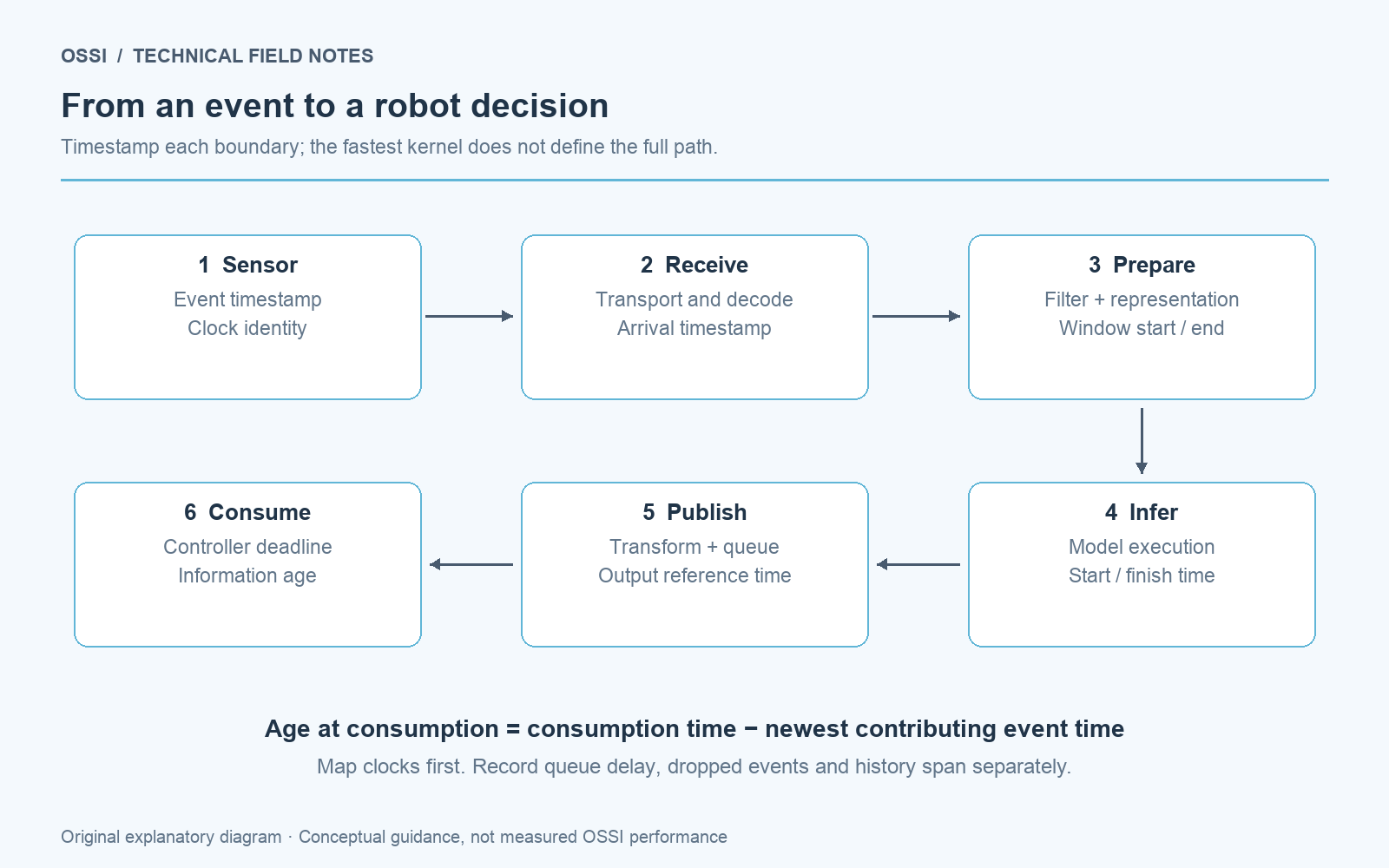
Measure the information age at the robot's decision point, alongside the processing time of each stage.
Recent EventCV research provides a concrete integration example: its Jetson Orin AGX detector case study uses a 50 ms accumulation window and approximately 28 ms processing, while its library simplifies streaming and representation handling. Those are different quantities, each relevant to deployment. 1
For your pipeline, draw where data changes ownership. A driver thread, middleware queue and inference worker can each introduce delay. Draw where timestamps change meaning, too. A packet-arrival timestamp is not automatically equivalent to its oldest event timestamp. Preserve both when possible.
Distinguish processing time from information age
A useful timing record includes the first and last event contributing to an output, packet arrival, processing start, processing finish, publication and consumption. These let you separate computation from accumulated history and waiting.
For an output built from an interval, report both the age of its newest information and the span of history it uses. The former indicates freshness; the latter indicates temporal context. Neither alone completely describes the estimate. A motion model may deliberately use older evidence while predicting a current state, so also record the time to which the output refers.
newest-information age = consumption time - newest contributing event time
history span           = newest event time - oldest contributing event time
queue delay            = processing start - data-ready time
processing time        = processing finish - processing start
These expressions require timestamps mapped to a common clock. If they come from different clocks, establish an offset and check whether it changes during the session. Report remaining synchronisation uncertainty rather than treating negative or implausible durations as excellent performance.
As an illustrative example, not a measured OSSI result, a representation using 20 ms of history could spend 2 ms queued and 4 ms processing. Calling it a “4 ms perception system” would conceal the other timing contributions. The correct report shows the window, queue and processing separately, plus the actual age when the consumer reads the output.
Read research results with their experimental conditions
The following studies address different parts of the information path. The table makes their boundaries visible rather than ranking unlike experiments by a single headline number.
| Research | Experimental substrate and task | Useful finding | Boundary for a robotics decision |
|---|---|---|---|
| EventCV 1 | Jetson preprocessing and detector workflows; desktop localisation case study | Integration and data handling affect deployment | Library throughput is not closed-loop robot latency |
| EventShiftFlow 2 | Synthetic/recorded motion; single-axis Artix-7 prototype | Quantised motion can use a small fixed datapath | One-axis implementation; reported power is a tool estimate |
| Propeller sensing 3 | Recorded outdoor flights of two quadrotors | Periodic event structure provides frequency cues | Estimation evaluation does not demonstrate online formation control |
| AdaFuse-Det 4 | Low-light RGB/event detection benchmark | Complementary sensing improves this benchmark's detection metrics | No embedded runtime or robot-control evaluation |
| Depth uncertainty 5 | Synthetic training and MVSEC indoor depth evaluation | Confidence can rank useful predictions | Selected-pixel accuracy trades away coverage |
| Event-based tactile force 6 | Physical sensor, controlled indentations, desktop processing | Events support contact-deformation estimation | Downstream grasping and embedded deployment remain open |
These distinctions help formulate a testable design. A result about representation generation informs one stage. A result about force reconstruction informs a measurement interface. Neither settles whether the entire robot will complete more tasks within its energy budget.
Choose accumulation rules deliberately
A fixed-duration window gives the downstream system a predictable update opportunity. Its information content changes with scene activity: a quiet scene supplies fewer events than a rapid turn past a textured wall. A fixed-event-count window provides more consistent input volume but changes the time needed to collect it.
Both behaviours matter. A detector may fail because a short window contains insufficient structure, while a controller may fail because a count-based window takes too long during slow motion. A larger window can improve a local benchmark yet delay the information that the robot needs.
Test the window rule as an explicit parameter. Record accuracy, information age, event count, representation-build time and memory use across each operating condition. Do not tune only on the busiest clip. Include intervals with little motion and abrupt transitions into heavy activity.
A hybrid policy can impose both a maximum duration and a maximum event count. Specify what happens when either limit is reached, and attach the actual interval to the output. That enables the consumer to distinguish an estimate based on a full information budget from one based on a deadline-limited sparse input. Validate the policy with recorded sequences before introducing adaptive behaviour into a live robot.
Budget for bursts, not just average rates
Measure event arrivals over several time scales. A one-second average can hide a short burst that fills a queue, and a large queue can hide that overload from an average throughput report. At the decision point the consequence is often stale information, even when the model keeps producing outputs.
Capture maximum observed backlog, packet loss, processing utilisation and output age. Label maxima as observed under the tested workload. They are not mathematical worst-case guarantees. Include sudden camera rotations, vibration, lighting transitions and highly active scenes in the workload set when those occur in your application.
Decide an overload policy before benchmarking. A pipeline may process every event and accumulate delay, discard some inputs, reduce spatial resolution or keep only the latest complete representation. Each option changes what the algorithm sees. Count dropped information and evaluate task performance under that policy.
An illustrative capacity calculation can guide buffer sizing: if input exceeds service capacity by two million events per second for 10 ms, the additional backlog is 20,000 events. This arithmetic is a planning example, not a sensor specification. The decisive follow-up is how long your actual service takes to remove that backlog while new data continues arriving.
Treat preprocessing as part of the model
Filters, cropping, polarity handling, temporal bins and normalisation define the input distribution. Changing them after training can change the model's behaviour even if its weights remain identical. Store their settings alongside the model version.
For every filter, ask which events it removes and whether those events can carry task-relevant information. A noise rule that cleans a static clip may also suppress a small or distant moving object. Evaluate the filter by the downstream task, not simply by the attractiveness of the resulting image.
Profile representation generation separately from inference. Measure memory allocation, copies and data-layout conversions. A dense tensor can lose much of the stream's sparsity before it reaches an accelerator. Its shape, dtype and temporal depth then become material hardware choices.
Create a reproducibility check: the same recorded input and configuration should produce the same model input, or documented differences where nondeterminism is intentional. Keep a small fixture with expected event counts and checksums for each transformation. This makes it easier to diagnose whether a deployment regression comes from the sensor path, representation builder or trained network.
Use approximate motion only where the task permits it
A robot does not always need a dense, sub-pixel flow field. Some decisions need an approximate motion direction or a compact cue that triggers a more expensive estimator. Reducing output detail can make a hardware implementation practical, provided the task still receives enough information.
EventShiftFlow's prototype reports 24 µs scoring after an occupancy bin; its real-sequence evaluation uses 40 ms bins. This illustrates why datapath latency and temporal observation interval must be assessed together. 2
For an approximate motion front end, define the tolerated angular and magnitude errors at the task interface. Test crossing objects, overlapping projections, weak event activity and changing motion. Include a “no reliable estimate” output rather than forcing every interval into a velocity category.
Evaluate whether a coarse cue reduces downstream work without increasing missed decisions. A practical two-stage design might use the cue to select a region or schedule detailed processing. Its benefit depends on the complete scheduling policy, including false triggers. Benchmark the combined route and the original route on identical recordings. Approximation is useful when it removes work while preserving the application requirement; compact hardware alone does not establish that.
Extract dynamics without overstating observability
Events can expose periodic structure that is awkward to recover from sparsely sampled frames. Propeller sensing demonstrates this on five held-out recorded outdoor flight sequences, with frequency MAPE of 2.75% for connected-component clustering and 2.73% for HDBSCAN. The experiment measures a specific physical cue, not every component of relative robot state. 3
When a system estimates state from such a cue, write down the additional assumptions. Which dimensions are directly measured? Which rely on known geometry, a motion model or another sensor? Which are unobservable from the chosen image configuration? These questions prevent a good component result from becoming an unsupported system claim.
Keep intermediate outputs available during evaluation: detections, tracked regions, frequency estimates and state-filter updates. If position error grows, those records distinguish missed detections from incorrect dynamics or calibration. Report component error and final state error separately.
Test loss and recovery of the cue. A target can leave the field of view, become occluded or change apparent size. The estimator should indicate how old its last measurement is and how uncertainty changes while it predicts without new evidence. Reacquisition is part of the operating envelope, not a detail to remove from the test set.
Compare fusion against meaningful alternatives
Adding an event sensor to an RGB pipeline introduces calibration, synchronisation and additional computation. Its value should be tested against several alternatives: the existing RGB system, a sensibly improved RGB system, an event-only model and the proposed fusion route. Keep splits and scoring rules consistent.
AdaFuse-Det reports low-light benchmark gains from RGB/event fusion. Its paper also identifies slow-motion cases where event cues weaken; it does not report an embedded deployment benchmark. 4
Build a condition matrix separating illumination from motion. Include dim scenes with fast movement, dim scenes with slow movement, bright scenes with movement and stationary targets. Otherwise an aggregate metric can conceal the conditions in which the added sensor helps or hurts.
Measure fusion overhead at the actual deployment resolution. Record calibration drift, missing packets and modality delay. Test how the system behaves when one modality is absent or unreliable. A learned fusion weight is not automatically a calibrated probability that the resulting detection is correct.
For each condition, report false positives and false negatives in operational terms. A change in F1 is useful, but a robot team also needs to know whether it represents fewer missed pedestrians, more nuisance stops or altered detection distance.
Pair uncertainty with coverage
An uncertainty estimate is valuable when it helps the consumer decide which predictions to use. It must be evaluated as part of that selection rule. Report how error changes as predictions are rejected, and how much of the scene remains covered.
Recent event-depth research finds that selecting low-uncertainty pixels reduces depth error, while its depth-only baseline achieves better overall RMSE. Confidence-aware prediction therefore requires an explicit accuracy–coverage trade-off. 5
A navigation system may need information in a particular region, not merely a low average error among the pixels retained elsewhere. Check coverage of the robot's intended path, thin structures and near objects. A confident estimate concentrated on easy background surfaces may leave the important region unresolved.
Evaluate confidence ranking on held-out operating conditions. A model can assign useful uncertainty within familiar indoor data yet behave differently after changes in lighting, texture or motion. Decide what the consumer does when required regions have insufficient evidence: request another sensor update, slow a manoeuvre or use a separately validated fallback.
Keep those actions separate from claims of safety. A confidence map and a rejection rule are components of a larger assurance process. Their practical value comes from tested behaviour at the application interface.
Carry the same questions into event-based touch
The same timing discipline applies when an event camera looks at a deformable tactile surface. Sensor changes must become displacement, force or slip-related information before a manipulation controller can act.
A recent tactile study reconstructs force from physical indentation data, with approximately 100 Hz processing on a desktop CPU/GPU. Dense predictions are assessed through measured net force; closed-loop manipulation is left for future work. 6
For a gripper application, test sustained contact as well as changing contact. Specify what remains available when the surface stops moving. Include material changes, repeated loading, calibration shifts and different contact geometries. Verify that force estimates retain meaningful units throughout the interface.
Evaluate the feedback loop after validating the sensor. Faster force estimates may help only if transport, controller scheduling and actuator response allow the robot to use them. A reconstruction benchmark should be followed by task measurements such as object retention, placement error or contact-force excursions, chosen for the intended application.
Use a worksheet that connects evidence to a buying decision
Complete this worksheet before requesting an accelerator benchmark or committing to sensor integration. Each entry should be backed by a recording, configuration or stated requirement.
- Task: Which decision must improve, and what current failure motivates the change?
- Envelope: What combinations of illumination, camera motion, target motion and contact occur?
- Data: Which representative recordings and independently labelled test sequences are available?
- Timing: What deadline, observation interval and maximum acceptable information age apply?
- Inputs: What timestamp format, calibration, filtering and synchronisation are required?
- Load: Which average and burst event rates were observed, with what loss and backlog?
- Outputs: Which estimate, units, confidence, validity flag and reference time reach the consumer?
- Comparison: Which existing and improved baselines use the same operating conditions?
- Resources: What host-inclusive compute, memory, energy and thermal budgets apply?
- Acceptance: Which task metrics and failure conditions determine whether integration is worthwhile?
Run the comparison in stages: reproducible replay, live sensing without control authority, and controlled task evaluation once interfaces and failure handling are understood. Archive both successful and failed sequences. The strongest report explains where the new information improved the task and where the original system remained preferable.
For the wider measurement framework, see How to Benchmark Neuromorphic Edge Compute for Robotics. For integration choices, see Building a Heterogeneous Robot Compute Stack. The OSSI neuromorphic robotics guide connects the series.
If your team is evaluating an event stream for a specific robot, Discuss your robotics workload with OSSI. Share the sensor stream, decision deadline, energy budget, compute platform and success criteria so the discussion starts with an engineering requirement.
References
- Adam D. Hines, Michael Milford and Tobias Fischer (2026). The EventCV Library for Event-Based Robotic Vision. arXiv:2609.21330v1; first released 18 September 2026. Preprint, under review according to the arXiv record.
- Arianna Alonso Bizzi, Fernando Cladera and C. J. Taylor (2026). EventShiftFlow: Towards Hardware-efficient FPGA-based Flow Estimation. arXiv:2605.28312v1; first released 27 May 2026. Accepted ICRA 2026 workshop paper; formal publication date not established here.
- Ravi Kumar Thakur, Luis Granados Segura, Jan Klivan, Radim Špetlík, Tobiáš Vinklárek, Matouš Vrba and Martin Saska (2026). Relative State Estimation using Event-Based Propeller Sensing. arXiv:2604.18289v1; first released 20 April 2026. Preprint, also listed among accepted ICRA 2026 workshop papers; formal publication date not established here.
- Raju Imandi, Chethana B, Bharatesh Chakravarthi, Yong-Guk Kim, Manipriya S and Pavan Kumar B N (2026). AdaFuse-Det: Adaptive Cross-Modal Fusion of Event Cameras for Robust Object Detection in Low-Light RGB Imagery. arXiv:2605.24691v1; first released 23 May 2026. Preprint, also listed among accepted ICRA 2026 workshop papers; formal publication date not established here.
- Viktor Bergkvist, Felix Rydell, Per-Erik Forssén, David Gustafsson and Johan Rideg (2026). Neuromorphic Monocular Depth Estimation with Uncertainty Modeling. arXiv:2605.10675v1; first released 11 May 2026. Preprint, also listed among accepted ICRA 2026 workshop papers; formal publication date not established here.
- Agis Politis, René Zurbrügg and Valentina Cavinato (2026). Dense Force Estimation with an Event-based Optical Tactile Sensor. arXiv:2606.09451v1; first released 8 June 2026. Preprint; formal peer-reviewed publication not established here.
Discuss your robotics workload with OSSI
Tell us about your platform and where adaptive, event-driven compute could help.
Start the conversation →