Continual Learning on the Robot: What Can Adapt On-Device Today?
Contents
- Define the adaptation job before choosing a learning rule
- What the recent evidence actually demonstrates
- Put a visible boundary around the plastic part
- Feedback is a sensor with its own failure modes
- Budget learning state and future growth
- Measure adaptation without hiding inference delays
- A practical adaptation protocol
- Read the learning curve as an operating record
- Adaptation-readiness worksheet
- When full representation learning is the next problem
- References
A robot deployed in a warehouse rarely encounters exactly the world represented by its training set. Packaging changes, lighting varies, a new tool appears and operators use unfamiliar gestures. Sending every change through a central retraining process can make adaptation slow. Allowing arbitrary updates on the robot, however, creates a different engineering problem: the machine may learn today's examples while becoming worse at yesterday's work.
The useful question is therefore specific: which part of the system can change, using which feedback, within what memory and timing budget, while retaining which capabilities? Recent neuromorphic research provides credible answers for selected learning components. It does not yet provide a universal recipe for a robot that improves continuously throughout its entire perception and control stack.
This article develops a practical evaluation method for robotics teams considering on-device adaptation. The research reviewed here was first released between 8 October 2025 and 8 October 2026. Preprints are identified as such. The proposed engineering workflow is guidance for an evaluation, rather than a claim about measured OSSI performance.
Define the adaptation job before choosing a learning rule
Several capabilities are commonly grouped under “learning on the robot”, although they demand different evidence.
Calibration adjusts parameters such as offsets, thresholds or sensor alignment. Its target is usually specified, and the update does not necessarily add new semantic knowledge. Online learning updates a model as samples arrive. It describes the timing of updates, but does not establish that previous tasks remain usable. Continual learning addresses acquiring new knowledge while retaining useful earlier knowledge under a defined sequence of experiences. Temporal state stores recent context during inference; a changing membrane potential or recurrent state is not, by itself, a learned parameter update.
These distinctions affect the purchase decision. If a gripper's problem is a drifting force offset, a controlled calibration routine may be sufficient. If an inspection station needs to recognise new packaging categories, adding class representations to a frozen feature extractor may be worth investigating. If changing material appearance makes the original visual features uninformative, adapting only the classifier may fail regardless of how efficiently that classifier learns.
Write the requirement as an observable change. For example: “After an authorised operator introduces a new component category, recognise it under the agreed lighting conditions while retaining the existing categories.” Then specify the available labels, acceptable introduction effort, update deadline and retention test. Avoid requirements such as “become more intelligent over time”, which cannot select an implementation or establish acceptance.
Separate learning from action authority. An adaptive perception component can produce a candidate label, confidence or novelty flag for an existing decision process. Evaluating this component does not require granting it unrestricted control of a robot. Start with the smallest adaptation boundary that can solve the identified problem.
What the recent evidence actually demonstrates
The following studies address different pieces of that boundary. The table is an evidence map, not a performance ranking: its workloads, precision and measurement scopes differ.
| Research | Experimental conditions | Demonstrated capability | Boundary for a robotics buyer |
|---|---|---|---|
| CLP-SNN 1 | OpenLORIS; measured Intel Loihi 2 learning head; frozen external feature extractor | Few-shot retention; hardware freezes prototypes after allocation | Head measurements exclude feature extraction and I/O; errors allocate additional prototypes |
| CLANE 2 | Recorded event-camera action clips; measured Loihi 2 pipeline; frozen pretrained spiking features | Class-incremental action recognition | Feature extraction is on-chip, but its weights remain frozen |
| Spiker-LL 3 | FPGA-targeted fixed-point design; supervised digit/image training | Local weight-update support | Power is tool-estimated; continual retention is not established |
| SpikON 4 | Supervised VGG11 training; ASIC synthesis and performance simulation | Training dataflow and reuse | Accelerator evidence does not show fabricated silicon or continual retention |
| DELL 5 | Dense event vision; off-chip FP32 GPU experiments | Block-wise learning with reduced training memory | Not demonstrated on-chip; temporal backpropagation remains within blocks |
CLP-SNN's current table reports 0.33 ms and 0.05 mJ per single-sample inference-and-update cycle in the learning head on Loihi 2. These are component measurements, not the energy or response time of a complete robot. 1
CLANE extends the investigation to event-based actions, moving feature extraction onto the same neuromorphic substrate. Its pretrained representation still constrains what the adaptive head can learn. 2
This research includes OSSI co-founder Yulia Sandamirskaya as a co-author; its experiments use Intel Loihi 2, not OSSI hardware. This disclosure applies to CLP-SNN and CLANE.
The practical implication is to evaluate learning location and learning capability separately. A model may execute entirely on a device while only one part of it changes. Conversely, an algorithm may reduce training memory in software without having a deployable hardware learning implementation.
Put a visible boundary around the plastic part
A useful starting architecture is a stable feature extractor followed by a small adaptive component. The stable part transforms sensor input into a representation. The plastic part associates that representation with classes, prototypes or another bounded output. An update policy decides when feedback is sufficient to change it.
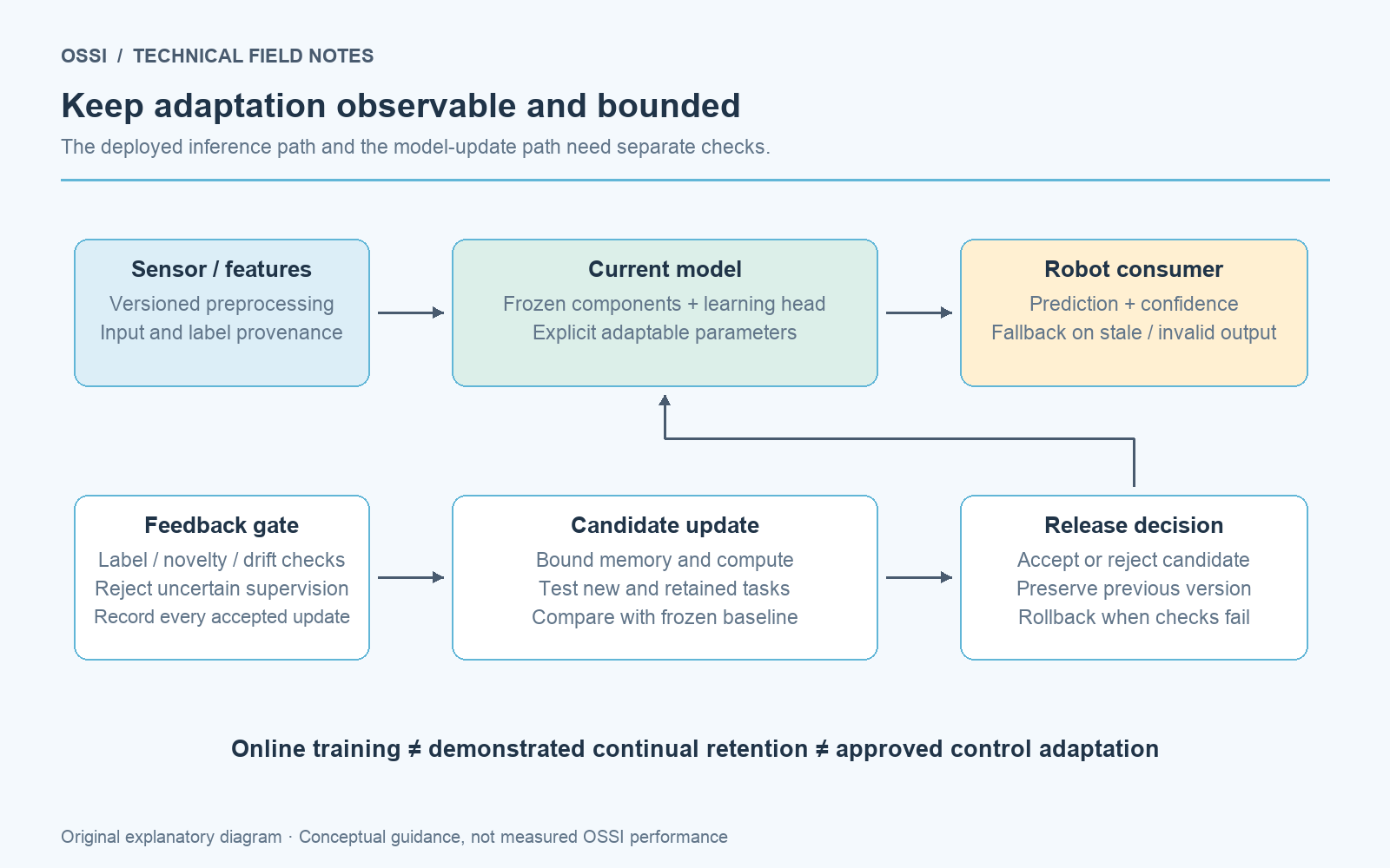
An evaluation architecture that makes the learning boundary, feedback source and promotion decision explicit. This is an original conceptual diagram, not a diagram of an OSSI product.
This separation is attractive because it limits the state that must be stored, compared and rolled back. It also creates a diagnostic question: do the existing features separate the new cases? Plot or inspect distances between labelled examples before building an elaborate learning controller. If old and new categories occupy nearly identical feature regions, changing the head may simply move errors between categories.
Test representation sufficiency with held-out examples from the intended operating conditions. Include visually similar existing categories and inputs outside the permitted adaptation task. A head that memorises one example is not necessarily learning a useful category. Multiple views of the same physical item should not all appear on both sides of the train/test boundary.
Freeze the interface as well as the weights. Document feature dimensions, scaling, normalisation, precision and version. Updating an upstream preprocessing step can move the feature space even if the neural backbone file remains unchanged. The deployed head then interprets values under assumptions that no longer hold.
If a backbone replacement is necessary, treat it as a separate release. Existing prototypes may require rebuilding or compatibility testing. Avoid assuming that a convenient parameter-file format makes learned representations interchangeable across versions.
Feedback is a sensor with its own failure modes
Every adaptive system needs an answer to “how does it know the update is right?” An operator label, a task outcome, a second sensor and a model-generated pseudo-label carry different uncertainty. Their provenance belongs in the experiment record.
For operator feedback, define who may label, which categories they may introduce and whether they can correct earlier labels. Give ambiguous examples an explicit unresolved state. For task feedback, examine delay and attribution: a failed grasp might originate in localisation, friction, motion planning or an actuator fault. Assigning the entire failure to a visual classifier can teach the wrong association.
A high-confidence prediction should not automatically become ground truth. That creates a feedback loop in which the model reinforces its existing errors. If pseudo-labels are used, keep their identity separate from independently verified labels and assess them against a reference set.
Specify the update unit. Is feedback attached to one event, one image, an action clip or a complete operation? It must identify the relevant input interval, not merely the wall-clock time when an operator pressed a button. Otherwise a delayed label can be applied to the next object in the stream.
Build a small feedback record containing the sample identifier, sensor interval, label or reward, source, verification state and model version. Keep this record compact if full raw-data storage is constrained. Record rejected updates as well as accepted ones; they reveal whether the system is ignoring an entire operating condition.
A useful gate checks that the input belongs to the agreed adaptation scope, the feedback is eligible and the update fits the current resource budget. The precise rules are application choices. Document them before testing so that a good result cannot be explained afterwards by selectively excluding difficult examples.
Budget learning state and future growth
An inference model's parameter count understates the memory required to learn. Depending on the method, add writable weights, learning-rate state, traces, optimiser state, replay samples, labels, temporary activations and candidate copies. Include metadata and alignment overhead rather than calculating only the payload bits.
Prototype methods make growth particularly visible. A new concept may require additional representations, and nuisance variation can create multiple representations of what the operator considers one category. Reserve capacity, define an exhaustion response and measure growth per operating hour or per accepted update.
Capacity exhaustion should produce a predictable outcome. Options include declining further additions, requesting consolidation or switching to an approved fixed configuration. Silently evicting old representations introduces an unmeasured retention policy. Consolidation itself needs evaluation: merging nearby prototypes might remove distinctions that matter operationally.
For an illustrative budget, suppose an adaptive head stores 256 prototypes, each with 512 eight-bit features. The raw prototype payload is 131,072 bytes, or 128 KiB. Doubling capacity doubles that payload before adding labels, state or routing. These figures are arithmetic examples, not measurements of OSSI or any cited implementation.
learning memory budget = writable parameters
                       + update state
                       + retained examples, if used
                       + growth reserve
                       + candidate and rollback state
                       + transport and alignment overhead
Writable storage also changes the hardware schedule. Spiker-LL illustrates a local-learning implementation whose memory and control architecture must support updates; it does not establish retention during a robot's long deployment. 3
Budget the feedback transport too. A compact reward signal may be cheap to transmit, while dense supervision for every pixel requires a different data path. Label granularity is an architectural decision, not simply a training preference.
Measure adaptation without hiding inference delays
The relevant deadline is normally the time until a useful decision is available. An update that is individually fast can still delay inference by contending for memory, blocking a queue or waiting for a label.
Measure three modes: inference with learning disabled, inference with learning enabled but no accepted updates, and inference during sustained eligible updates. This separates the cost of maintaining the learning machinery from the cost of actually changing parameters. Repeat during sensor bursts and under competing robot workloads.
Record decision latency, update completion time and queue age independently. “One sample processed per millisecond” is incomplete if a queue has already accumulated stale samples. A robot observing a changed scene needs a current decision, not merely high throughput on an old stream.
Define update scheduling around the task. A calibration period, an idle interval and continuous adaptation impose different requirements. A deferred update may be acceptable if the robot can continue with its existing model, but the delay becomes part of the adaptation service level.
SpikON investigates supervised learning dataflow rather than a continual-retention protocol. Its accelerator estimates motivate attention to scheduling and memory reuse, but do not prove those gains on a deployed robot. 4
Energy should cover the agreed learning interval and include the accompanying host work. Report the energy of a successful accepted update and the total energy consumed while waiting, rejecting examples and maintaining state. If labels are supplied remotely, distinguish on-device execution from the connectivity required to sustain the feedback process.
A practical adaptation protocol
Use a chronological experiment rather than a shuffled dataset to assess continual learning. Shuffling can hide the distribution changes that the system is meant to handle.
1. Establish the fixed baseline. Run the current model on representative recorded streams. Measure task quality, latency, memory and power using the same configuration planned for the adaptive candidate. Preserve difficult examples and existing failure cases. They become useful controls when diagnosing apparent improvements.
2. Define the experience sequence. Construct sessions containing existing categories, new categories, returning categories and changed conditions. Include a period with no legitimate new knowledge. This checks whether the method unnecessarily changes a stable model. Use several session orders so that success does not depend on a favourable introduction sequence.
3. Separate update data from evaluation data. Hold out different physical instances, recording sessions and relevant conditions. Keep an earlier-task test bank that the learner does not consume. If a replay-based method is compared, its permitted training buffer must be distinct from this evaluation bank.
4. Evaluate before updating. Score each incoming labelled sample with the current state, then permit the eligible update. This records what the system knew before receiving the answer. Testing only after an update can make memorisation appear as predictive capability.
5. Evaluate retention after each introduction. Test the new task and previously introduced tasks. Report per-category outcomes, not only their average. A large easy category can conceal the disappearance of a small operationally important one. Measure both current accuracy and the decline from each earlier task's best observed performance.
6. Stress feedback and resources. Add controlled missing labels, delayed labels and incorrect feedback. Fill the growth reserve, vary input density and interrupt the learning process. Check that a partial update does not leave the model in an undocumented state. These tests assess the proposed implementation, rather than extrapolating from a paper's nominal benchmark.
7. Run the candidate in shadow mode. Feed live streams to the candidate while an established path remains responsible for decisions. Compare outputs using independently reviewed outcomes. Investigate disagreement episodes, including confident disagreements and novelty flags on familiar inputs. Log enough context to reproduce them.
8. Promote a versioned candidate. Require the agreed new-task improvement, retention floor and resource limits to pass together. Save the candidate's identifier, parameters and compatible preprocessing version. Preserve the prior state and demonstrate that restoration works. Promotion can be a controlled release even if the learning itself occurred locally.
This protocol gives the engineering team a defensible answer when adaptation fails. Poor new-task performance, excessive forgetting, unreliable feedback and resource exhaustion become separate findings, each requiring a different remedy.
Read the learning curve as an operating record
A final score compresses the sequence that produced it. Plot performance against accepted updates and elapsed operating time, then annotate category introductions, changed conditions and capacity events. These views reveal whether an improvement requires an impractical amount of operator effort or arrives only after a long period of poor decisions.
Track abstention and coverage alongside accuracy. A candidate can appear more accurate by declining unfamiliar inputs; that may be useful, but it changes the service it provides. Record the fraction of inputs for which it produces an eligible decision and the workflow used when it declines.
Distinguish forgetting from increasing task difficulty. Adding similar classes can make classification harder without erasing earlier representations. A per-task retention bank helps locate the affected categories, while confusion matrices show whether failures concentrate around new competitors. Preserve these records so that the next model revision can target an identifiable problem instead of optimising one overall number.
Adaptation-readiness worksheet
Complete this worksheet before an implementation sprint. Empty cells are unresolved design requirements.
| Decision | Record for the proposed workload |
|---|---|
| Adaptation target | Exactly which categories, parameters or behaviours may change? |
| Plastic boundary | Which weights and state are writable; which components are frozen? |
| Input contract | Sensor interval, preprocessing version, feature scale and precision |
| Feedback contract | Source, eligibility, delay, correction procedure and sample association |
| Retention requirement | Per-task floor and permitted decline on earlier tasks |
| Growth budget | Maximum writable state, reserve and exhaustion response |
| Timing budget | Decision deadline, update interval and maximum queue age |
| Energy budget | Measurement boundary, operating modes and update frequency |
| Promotion rule | Required quality/resource outcomes and candidate owner |
| Restoration | Prior state, compatibility checks and demonstrated rollback |
Make the worksheet part of the evaluation report. A demonstrator that cannot answer these questions may still be scientifically useful, but it does not yet give an OEM sufficient information to integrate the learning behaviour.
When full representation learning is the next problem
If the frozen representation is inadequate, the next step is deeper adaptation. That introduces intermediate activations, error propagation, additional supervision and a larger set of changing parameters. The deployment problem becomes considerably broader.
DELL offers a recent example of progress towards local dense-vision training, with a reported 39.6% peak training-memory reduction against its matching end-to-end reference. Its experiments use off-chip FP32 GPUs; the paper explicitly leaves on-chip training and silicon validation unresolved. 5
For an engineering programme, this is a reason to separate two milestones: showing that a learning method works on the target data, and showing that the entire update procedure fits the intended device. Passing the first does not automatically pass the second.
Choose the smallest plastic region that addresses the real source of failure. Expand it only when held-out evidence shows that its representational limits are the bottleneck. That approach produces clearer experiments, more predictable resource budgets and a more useful conversation between robotics and hardware teams.
For the wider selection process, use the OSSI neuromorphic robotics guide. Pair this article with How to Benchmark Neuromorphic Edge Compute for Robotics and Deploying Spiking Neural Networks on FPGA.
Bring your sensor stream, decision deadline, energy budget, compute platform and success criteria. Discuss your robotics workload with OSSI.
References
- Elvin Hajizada, Danielle Rager, Timothy Shea, Leobardo Campos-Macias, Andreas Wild, Eyke Hüllermeier, Yulia Sandamirskaya and Mike Davies (2026). Online Continual Learning on Intel Loihi 2 via a Co-designed Spiking Neural Network. arXiv:2511.01553v2, version dated 5 May 2026; first public release 3 November 2025. Preprint; this article uses v2. Full text.
- Elvin Hajizada, Michael Neumeier, Edward Paxon Frady, Yulia Sandamirskaya, Axel von Arnim, Bing Li and Eyke Hüllermeier (2026). CLANE: Continual Learning of Actions on Neuromorphic Hardware from Event Cameras. arXiv:2605.28387v1; first public release and version date 27 May 2026. Preprint. Full text.
- Alessio Caviglia, Filippo Marostica, Alessandro Savino and Stefano Di Carlo (2026). Spiker-LL: An Energy-Efficient FPGA Accelerator Enabling Adaptive Local Learning in Spiking Neural Networks. arXiv:2605.18003v1; first public release and version date 18 May 2026. Preprint. Full text.
- Peilin Chen and Xiaoxuan Yang (2026). SpikON: A Dual-Parallel and Efficient Accelerator for Online Spiking Neural Networks Learning. arXiv:2606.30926v1; first public release and version date 29 June 2026. arXiv records acceptance to ISLPED 2026; the cited version is the preprint. Full text.
- Maxime Vaillant, Axel Carlier, Lai Xing Ng, Christophe Hurter and Benoit R. Cottereau (2026). Toward On-Chip Training of Spiking Neural Networks for Dense Event-Based Vision. arXiv:2609.32405v1; first public release and version date 26 September 2026. Preprint. Full text.
Discuss your robotics workload with OSSI
Tell us about your platform and where adaptive, event-driven compute could help.
Start the conversation →